Logistic Regression

Logistic Regression

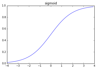
logistic regression 和 perceptron 其实是比较像的,都是只能对线性可分的数据建模,也是基于神经科学的神经元模型得来的,神经元模型图如下。不过 logistic regression 的输出结果值具有一定的解释性,可以把它理解为概率。另外一方面,logistic regression 可以很容易地扩展到对多个类建模,而 percptron 只能作为二元分类器。 logistic regression 使用 sigmoid 激活函数

\[\sigma = \frac{1}{1 + \exp^{-z}}\]

如果更加深入的来说,对于输入为\(x_1,x_2,x_3,...\),权重为\(w_1,w_2,w_3,...\),偏置\(b\),则相对应的激活值为

\[\frac{1}{1 + \exp^{- \sum_i{w_ix_i} - b}}\]

神经元模型

学习准则

学习到的模型需要一个机制去评估参数\(w,b\)是否比较好,所以说需要对我们做出的模型函数进行评估,一般这个函数称为损失函数(loss function)或者错误函数(error function)。假设模型拟合函数为\(h(\theta)\),那么在我们这个 logistic regression 模型中有\(h(\theta)=\sigma(w,b)\).描述模型函数\(h(\theta)\)不好的程度,一般称这个函数为损失函数,通常情况下可以使用欧氏距离损失函数 \[J(\theta)=\frac{1}{2} \sum_i^N{(h_{\theta}(x^i) - y^i)^2}\] 只要最优化这个函数便可以得到在这个损失函数标准下的最好的模型。在机器学习方法中通常使用迭代的方法来逼近最有解,所以在这个算法里也使用了同样的思想。

梯度下降

在选定线性回归模型后,只需要确定参数\(\theta\),就可以将模型用来预测。然而θ需要在 \(J(\theta)\)最小的情况下才能确定。因此问题归结为求极小值问题,使用梯度下降法。梯度下降法最大的问题是求得有可能是全局极小值,这与初始点的选取有关。 梯度下降法是按下面的流程进行的:

  1. 首先对\(\theta\)赋值,这个值可以是随机的,也可以让\(\theta\)是一个全零的向量。
  2. 改变\(\theta\)的值,使得 \(J(\theta)\)按梯度下降的方向进行减少。

梯度方向由 \(J(\theta)\)\(\theta\)的偏导数确定,由于求的是极小值,因此梯度方向是偏导数的反方向。结果为

\[\theta_j := \theta_j + \alpha(h_{\theta}(x^i - y^i))x_j^i\]

迭代更新的方式有两种,一种是批梯度下降,也就是对全部的训练数据求得误差后再对θ进行更新,另外一种是增量梯度下降,每扫描一步都要对θ进行更新。前一种方法能够不断收敛,后一种方法结果可能不断在收敛处徘徊。这次实现的算法中使用的是批梯度下降的方法。

Logistic Regression 背后的概率原理

logistic regression 是人工神经网络中非常基础也是非常重要的一个模型,就算是深度学习中的深度神经网络中的决策层也 是经常使用 logistic 层或者softmax层。在网上搜索基本上很少看到 有分析 logistic regression 原理性的中文博客文章,大多是直接上公式然后求梯度,只解释了怎么用,而不解释清楚什么情 况下可以用,为什么可以用,所以打算再深入的剖析 logistic regression 背后合理性,也加强自己的记忆。我们可能会问, 为何可以用\(\sigma\)函数来做回归,并且符合哪些分布的数据用 logistic regression 能够得到较好的效果。 为了分析的简单,先分析两类的情况,其实也很容易拓展到多类。假设在每个类的条件下数据分布的密度函数为 \(p(\mathbf{x}|\mathcal{C}_k)\),每个类的先验概率为\(p(\mathcal{C}_k)\),那么我们的任务就是使用贝叶斯公式计算后验概 率\(p(\mathcal{C}_k|\mathbf{x})\).由于我们只考虑两类的情况,对于类\(\mathcal{C}_1\)的后验概率可以写为

\[ \begin{aligned} p(\mathcal{C}_1|\mathbf{x}) &= \frac{p(\mathbf{x}|\mathcal{C}_1) p(\mathcal{C}_1)} {p(\mathbf{x}|\mathcal{C}_1) p(\mathcal{C}_1) + p(\mathbf{x}|\mathcal{C}_2) p(\mathcal{C}_2)} \\ &= \frac{1}{1 + \exp(-a)} = \sigma(a) \end{aligned} \]

其中\(a\)是一个非常关键的参数,整个模型都由这个参数来决定,定义为

\[ a = \ln{\frac{p(\mathbf{x}|\mathcal{C}_1) p(\mathcal{C}_1)}{p(\mathbf{x}|\mathcal{C}_2) p(\mathcal{C}_2)}} \]

\(\sigma(a)\)就是 logistic sigmoid 函数,定义为\(\sigma(a) = \frac{1}{1 + \exp(-a)}\)很容易验证 logistic sigmoid 函数的逆为\(a = \ln(\frac{\sigma}{1-\sigma})\) 这其实是一个logit function,表示两个类概率比率的对数\(\ln[p(\mathcal{C}_1|\mathbf{x})/p(\mathcal{C}_2|\mathbf{x})]\) 对于多个类,也很容易得到每一个类的后验概率

\[ \begin{aligned} p(\mathcal{C}_k | \mathbf{x}) &= \frac{p(\mathbf{x}|\mathcal{C}_k) p(\mathcal{C}_k)} {\sum_j{p(\mathbf{x}|\mathcal{C}_j) p(\mathcal{C}_j)}} \\ &= \frac{\exp(a_k)}{\sum_j{\exp(a_j)}} \end{aligned} \]

其中\(a_k\)

\[ a_k = \ln p(\mathbf{x}|\mathcal{C}_k) p(\mathcal{C}_k) \]

其实这个函数也就是 softmax 函数。

从上面的分析看,对于两类的情况(多类也同理),每个类的后验概率就是 logistic sigmoid 函数,单\(a\)是线性的时候,也就是\(a = \ln{\frac{p(\mathbf{x}|\mathcal{C}_1) p(\mathcal{C}_1)}{p(\mathbf{x}|\mathcal{C}_2) p(\mathcal{C}_2)}}\)是线性时,我们便可以使用 logistic regression 来对数据集做回归分析,这样就能得到很好的效果。这样说可能还有点模糊,因为我们很难知道一个分布中\(a = \ln{\frac{p(\mathbf{x}|\mathcal{C}_1) p(\mathcal{C}_1)}{p(\mathbf{x}|\mathcal{C}_2) p(\mathcal{C}_2)}}\)是不是线性的,其实只要是指数族分布就可以用 logistic regression 来做回归,这里就不解释原因了,具体可以参考 Christopher M. Bishop 的Pattern Recognition And Machine Learning

sigmoid 激活函数如下图

sigmoid.png

代码实现

1
2
3
4
5
6
7
8
9
10
11
12
13
14
15
16
17
18
19
20
21
22
23
24
25
26
27
28
29
30
31
32
33
34
35
36
37
38
39
40
41
42
43
44
45
46
47
48
49
50
51
52
53
54
55
56
57
58
59
60
61
62
63
64
65
66
67
68
69
70
71
72
73
74
75
76
77
78
79
80
81
82
83
84
85
86
87
88
89
90
91
92
93
94
95
96
97
98
99
100
101
102
103
104
105
106
107
108
109
110
111
112
113
114
115
116
117
118
119
120
121
122
123
124
125
126
127
128
129
130
131
132
133
134
135
136
137
138
#! /usr/bin python

from __future__ import print_function
from __future__ import division
import random
import numpy as np
import cPickle as pkl

__author__ = 'wangzx'

class LogisticRegression(object):

def __init__(self, dim, n_class=2):
self.n_class = n_class
self.dim = dim
self.biases = np.random.randn(n_class, 1)
self.weights = np.random.randn(n_class, dim)

def feedforward(self, x):
fd = sigmoid(np.dot(self.weights, x)+self.biases)
return fd / np.sum(fd)

def SGD(self, training_data, epochs, mini_batch_size, eta,
test_data=None):

"""使用 mini-batch stochastic gradient descent 方法训练网络。
``training_data``是一个列表元组``(x,y)``,代表训练的输入和目标输出。
如果提供``test_data``的话,在每一个 epoch 完成之后会用模型计算这个数据相对应的
输出。这个可以让我们更清楚整个训练情况,不过会降低训练的速度。
"""

if test_data: n_test = len(test_data)
n = len(training_data)
for j in xrange(epochs):
random.shuffle(training_data)
mini_batches = [
training_data[k:k+mini_batch_size]
for k in xrange(0, n, mini_batch_size)]
for mini_batch in mini_batches:
self.update_mini_batch(mini_batch, eta)
if test_data:
print("Epoch {0}: {1} / {2}".format(
j, self.evaluate(test_data), n_test))
else:
print("Epoch {0} complete".format(j))

def update_mini_batch(self, mini_batch, eta):
"""通过随机梯度下降的方法来更新权值。
``mini_batch``是一个元组列表``(x,y)``,每一项是一个训练数据,分别代表
训练输入和目标输出,``eta``是学习率"""


# nabla_b 和 nabla_w 分别表示 b 和 w 的梯度
nabla_b = np.zeros_like(self.biases)
nabla_w = np.zeros_like(self.weights)

for x, y in mini_batch:
delta_nabla_b, delta_nabla_w = self.backprop(x, y)
nabla_b += delta_nabla_b
nabla_w += delta_nabla_w

self.weights -= eta / len(mini_batch) * nabla_w
self.biases -= eta / len(mini_batch) * nabla_b

def backprop(self, x, y):
"""其实可以不用写一个 backprop 函数,直接算梯度就行了,不过为了和 bp 神经网络
的代码结构尽量保持相似,所以也写了一个 backprop 函数"""

# feedforward
activation = self.feedforward(x)

# backward pass
delta = self.cost_derivative(activation, y) * \
sigmoid_prime(np.dot(self.weights, x) + self.biases)
return delta, np.dot(delta, x.T)

def evaluate(self, test_data):
"""返回预测准确的样本个数"""
test_results = [(np.argmax(self.feedforward(x)), y)
for (x, y) in test_data]
return sum(int(x == y) for (x, y) in test_results)

def cost_derivative(self, output_activations, y):
# 因为 y 是一个常数值,要转为 one-hot 编码
t = np.zeros((self.n_class, 1))
t[y, 0] = 1

#使用欧氏距离损失函数,其导数如下
return (output_activations-t)


#### Miscellaneous functions
def sigmoid(z):
"""sigmoid 函数."""
return 1.0/(1.0+np.exp(-z))

def sigmoid_prime(z):
"""sigmoid 函数的导数."""
return sigmoid(z)*(1-sigmoid(z))

def test():
feat = pkl.load(open("data/train_X.pkl", 'rb'))
#对数据进行归一化处理
feat = (feat - np.min(feat, axis=0)) / (np.max(feat, axis=0) - np.min(feat, axis=0) + 1e-3)
y = pkl.load(open("data/train_Y.pkl", 'rb'))
train_data = [(np.asarray(f).reshape((-1,1)), t) for f, t in zip(feat, y)]
test_feat = pkl.load(open("data/test_X.pkl", 'rb'))
test_feat = (test_feat - np.min(test_feat, axis=0)) / \
(np.max(test_feat, axis=0) - np.min(test_feat, axis=0) + 1e-3)
test_y = pkl.load(open("data/test_Y.pkl", 'rb'))
test_data = [(np.asarray(f).reshape((-1,1)), t) for f, t in zip(test_feat, test_y)]
n_sample, ndim = feat.shape
logistic = LogisticRegression(ndim)

print("Begin fit training data")
logistic.SGD(train_data, 50, 50, 0.01, test_data)

score = logistic.evaluate(test_data) / len(test_data)
print("Test accuracy is %f" % score)

def test_mnist():
path = '/home/wangzx/usr/share/data/mnist2/'
train_X = pkl.load(open(path + 'mnist_train_X.pkl'))
train_y = pkl.load(open(path + 'mnist_train_y.pkl')).ravel()
test_X = pkl.load(open(path + 'mnist_test_X.pkl'))
test_y = pkl.load(open(path + 'mnist_test_y.pkl')).ravel()
train_data = [(np.asarray(f).reshape((-1,1)), t) for f, t in zip(train_X, train_y)]
test_data = [(np.asarray(f).reshape((-1,1)), t) for f, t in zip(test_X, test_y)]
n_sample, ndim = train_X.shape
logistic = LogisticRegression(ndim, n_class=10)

print("Begin fit training data")
logistic.SGD(train_data, 50, 50, 0.02, test_data)

score = logistic.evaluate(test_data) / len(test_data)
print("Test accuracy is %f" % score)

if __name__ == "__main__":
#test()
#test_mnist()
pass

当前网速较慢或者你使用的浏览器不支持博客特定功能,请尝试刷新或换用Chrome、Firefox等现代浏览器