感知器学习算法

2016-05-22

机器学习神经网络

感知器学习算法（PLA）

感知器学习算法（PLA）

Perceptron（感知器）这个词是机器学习中的一个重要概念，来源于神经科学，是科学家们通过数学的方法来模拟神经元的工作方式而得到的一种简单的机器学习算法。

神经元模型

对于神经元的简单抽象如图所示,每个神经元是与其他神经元连结在一起的，一个神经元会受到多个其他神经元状态的冲击，并且不同神经元传来的神经冲动对该神经元的影响不同，由一个加权因子 w 来控制，并由此决定自身激发状态。

在这个模型中神经元的激活值 a 表示为

\[a = \left[\sum_{d=1}^{D}{w_dx_d}\right]+b\]

这里的偏移量 b 也是有一定意义的：

定义了神经元的激发临界值
在空间上，它对决策边界(decision boundary) 有平移作用，就像常数作用在一次或二次函数上的效果

感知器算法

感知器使用特征向量来表示的前馈式人工神经网络，它是一种二元分类器，把矩阵上的输入 x（实数值向量）映射到输出值 f(x)上（一个二元的值）。

\[ y= \begin{cases} 1, \quad \text{if} \,\,\, wx + b > 0\\ 0, \quad \text{else} \end{cases} \]

感知器算法是二维线性分类器(Binary Classifier)，但它与我们所知道的决策树算法和 KNN 都不太一样。主要区别在于：

感知器算法是一种所谓“错误驱动(error-driven)”的算法。当我们训练这个算法时，只要输出值是正确的，这个算法就不会进行任何数据的调整。反之，当输出值与实际值异号，这个算法就会自动调整参数的比重。
感知器算法是实时(online)的。它逐一处理每一条数据，而不是进行批处理。

学习准则

对于感知器学习算法来说，学习准则是比较简单的。只有判别错误的时候才进行更新，更新公式为：

\[ w \leftarrow w_d + yx_d \\ b \leftarrow b + y \]

具体实现

下面是感知器学习算法的具体实现。这个算法使用了两个测试数据，一个是老师提供的分类数据，一个是自动生成的多元高斯分布的数据。

#! /usr/bin python

from __future__ import print_function
import numpy as np
import matplotlib.pyplot as plt

__author__ = 'wangzx'

def generate_data(mean, cov):
    x = []
    y = []
    for i, m in enumerate(mean):
        x.extend(np.random.multivariate_normal(m, cov[i], (1000,)))
        y.extend([i] * 1000)
    g_data = [(f, t) for f, t in zip(x, y)]
    np.random.shuffle(g_data)
    return g_data

def plot_data(g_data, line=None):
    x = [f for f, t in g_data]
    x = np.asarray(x)
    y = [t for f, t in g_data]
    y = np.asarray(y)
    plt.scatter(x[:,0], x[:,1], 20, y)
    if line is not None:
        plt.plot(line[:,0], line[:,1], 'g')
    #plt.plot([-8,6], [-4, 14], 'g')
    plt.show()

def main():
    mean = [[-2,7], [1,1]]
    cov1 = [[1,0.5], [0.5, 3]]
    cov2 = [[1,0], [0,1]]
    g_data = generate_data(mean, [cov1, cov2])
    plot_data(g_data)

if __name__ == '__main__':
    main()

上面的脚本文件生成了包含两个类标的数据，每一类中的数据都是服从多元高斯分布的，数据如下图所示。

#! /usr/bin python

from __future__ import print_function
from __future__ import division
import numpy as np
import cPickle as pkl
from generate_data import generate_data, plot_data
__author__ = 'wangzx'


class Perceptron(object):
    """ A Perceptron instance can take a function and attempt to
    ``learn`` a bias and set of weights that compute that function,
    using the perceptron learning algorithm."""

    def __init__(self, inputs):
        """ Initialize the perceptron with the bias and all weights
        set to 0.0. ``inputs`` is the input to the
        perceptron."""
        num_inputs = inputs.shape[1]
        self.num_inputs = num_inputs
        self.bias = 0.0
        self.weights = np.zeros(num_inputs)
        self.inputs = inputs

    def output(self, x):
        """ Return the output (0 or 1) from the perceptron, with input
        ``x``."""
        return 1 if np.inner(self.weights, x)+self.bias > 0 else -1

    def learn(self, y, eta=0.1, max_epoch=100):
        # initialize the bias and weights with random values
        self.bias = np.random.normal()
        self.weights = np.random.randn(self.num_inputs)
        number_of_errors = -1
        epoch = 0
        while number_of_errors != 0 and epoch < max_epoch:
            number_of_errors = 0
            epoch += 1
            #print("epoch %d" % epoch)
            #print("Beginning iteration")
            for i, x in enumerate(self.inputs):
                y_pre = self.output(x)
                if y[i] != y_pre:
                    number_of_errors += 1
                    self.bias = self.bias + eta*y[i]
                    self.weights = self.weights + eta*y[i]*x
            #print("Number of errors:", number_of_errors, "\n")
    def predict(self, X):
        res = [self.output(x) for x in X]
        return np.asarray(res)
def test():
    feat = pkl.load(open("data/train_X.pkl", 'rb'))
    y = pkl.load(open("data/train_Y.pkl", 'rb'))
    y[y==0] = -1
    test_feat = pkl.load(open("data/test_X.pkl", 'rb'))
    test_y = pkl.load(open("data/test_Y.pkl", 'rb'))
    test_y[test_y==0] = -1
    pla = Perceptron(feat)

    print("Begin fit training data")
    pla.learn(y, eta=1)

    y_prd = pla.predict(test_feat)
    score = np.sum(y_prd == test_y) / y_prd.shape[0]
    print("Test accuracy is %f" % score)

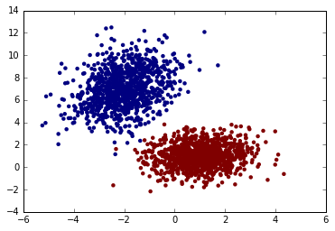
def test_gdata():
    mean = [[-2,7], [1,1]]
    cov1 = [[1,0.5], [0.5, 3]]
    cov2 = [[1,0], [0,1]]
    g_data = generate_data(mean, [cov1, cov2])
    X = [f for f, t in g_data]
    X = np.asarray(X)
    y = [t for f, t in g_data]
    y = np.asarray(y)
    y[y==0] = -1

    pla = Perceptron(X)
    print("Begin fit training data")
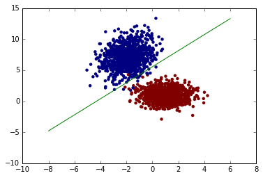
    pla.learn(y, eta=1, max_epoch=300)

    y_prd = pla.predict(X)
    score = np.sum(y_prd == y) / y_prd.shape[0]
    print("Test accuracy is %f" % score)
    border_line(pla, g_data)

def border_line(pla, g_data):
    b = pla.bias
    w = pla.weights
    x = np.asarray([[-8, 6]])
    y = -(w[0]*x + b) / w[1]
    plot_data(g_data, np.concatenate((x, y)).T)
if __name__ == "__main__":
    #test()
    #test_gdata()
    pass

这是在自动生成的数据集中得到的结果，可以看到感知器算法能够比较理想地拟合线性可分的数据（这个数据集并非是线性可分的，有几个数据点交叉了，所以要设定 max_epoch，而不是让它迭代直至收敛）。