Support Vector Machine

2016-05-23

机器学习

Support Vector Machine

Support Vector Machine

线性可分类

这里只介绍两类的线性可分问题，我们的任务就是设计一个超平面来划分数据集。设\(\mathbf{x}_i, i=1,2,\ldots,N\)是训练集\(X\)中的特征向量。这些类来自于类\(\omega_1, \omega_2\),并且假设是线性可分的。那么我们设计的超平面可以用这条公式来描述：

\[g(x) = \mathbf{\omega}^T \mathbf{x} + \omega_0\]

如果用感知器算法来解，可能会收敛到任何可能的解。而对于这样的问题，得到的超平面不是唯一的，如下面这幅图所示。

从上面的图来看，我们觉得用\(l_2\)这条线作为决策边界会更好一点。因为这条线把两个类分得比较开。基于这样的直觉，我们希望得到一条最优的分界线,而这条分界线是如何定义的，又是如何得到的，这就是 SVM 要解决的问题。

问题的定义与求解

基于上面的介绍，我们现在的任务就是寻找一个方向使得分界线使得间隔尽可能大(具体解释可参考 Simon Haykin 教授的Neural Networks and Learning Machines),因为平面到点的距离可以通过下面这条公式求解

\[z = \frac{|g(x)|} {\|\mathbf{w}\|}\]

因为缩放参数\(\omega\)不影响直线，现在缩放\(\omega, \omega_0\),使得点在\(\omega_1\)和\(\omega_2\)类中的间隔最近，\(g(x)\)对于\(\omega_1\)等于 1，对于\(\omega_2\)等于-1，因而有可以进一步把问题用下面的方程来表示：

存在一个间隔，满足\[\max_{\mathbf{w}} \frac{1}{\|\mathbf{w}\|}\]
要求满足约束

\[\mathbf{w}^T \mathbf{x} + w_0 \ge 1, \quad \forall \mathbf{x} \in \omega_1 \\ \mathbf{w}^T \mathbf{x} + w_0 \le -1, \quad \forall \mathbf{x} \in \omega_2 \]

对于每一个\(\mathbf{x}_i\),用\(y_i\)表示相对应的类标(对于\(\omega_1\)为+1，对于\(\omega_2\)为-1)，则现在可以简化为计算超平面参数\(\mathbf{w},w_0\):

\[\min_{(\mathbf{w}, w_0)} \mathcal{J}(\mathbf{w}, w_0) \equiv \frac{1}{2} \|\mathbf{w}\|^2 \\ \text{constraint to}. \quad y_i(\mathbf{w}^T\mathbf{x}_i + w_0) \ge 1, \quad i = 1,2,\ldots, N \]

具体的公式介绍和推导可参考下面两本教材和博客，里面有非常详细的推导 Simon Haykin 教授的Neural Networks and Learning Machines Sergios Theodoridis 教授和 Konstantinos Koutroumbas 教授的Pattern Recognition 支持向量机通俗导论

线性不可分问题

对于这个问题只把关键公式写出来，就不做详细分析了，主要想法就是引入松弛变量(slack variable)\(\xi_i\), 约束条件改为 \[y_i(\mathbf{w}^T \mathbf{x} + w_0) \ge 1 - \xi_i\] 最终解最小化代价函数

\[ \min \mathcal{J}(\mathbf{w}, w_0, \mathbf{\xi}) = \frac{1}{2} \|\mathbf{w}\|^2 + \mathcal{C} \sum_{i=1}^N {I(\xi_i)}\\ \text{subject to.} \quad y_i(\mathbf{w}^T \mathbf{x} + w_0) \ge 1 - \xi_i, \quad i=1,2,\ldots,N \\ \xi_i \ge 0, \quad i=1,2,\ldots,N \]

其中，\(\mathbf{\xi}\)是参数\(\xi_i\)组成的向量，并且

\[I(\xi_i) = \begin{cases} 1, \quad \xi_i \gt 0 \\ 0, \quad \xi_i = 0 \end{cases} \]

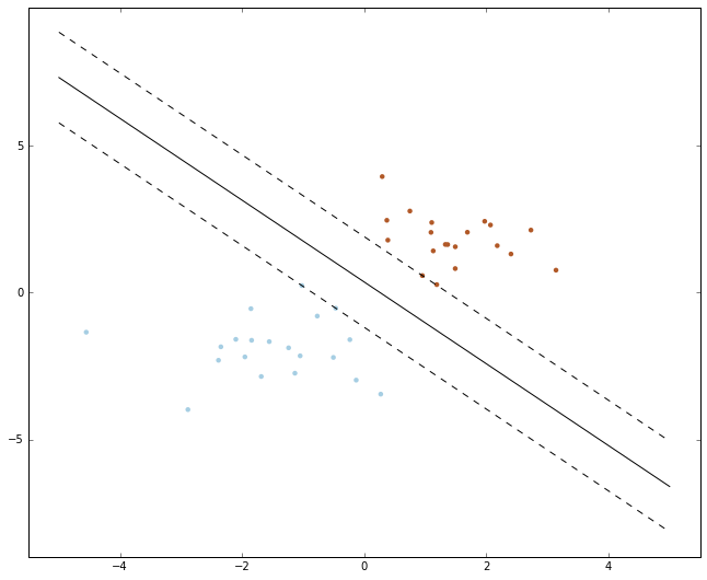
为了更清晰的了解支持向量机的工作机制，这里借用了 sklearn 中 svm 的例子，具体可参考svm margin example

import numpy as np
import matplotlib.pyplot as plt
from sklearn import svm

# we create 40 separable points
np.random.seed(0)
X = np.r_[np.random.randn(20, 2) - [2, 2], np.random.randn(20, 2) + [2, 2]]
Y = [0] * 20 + [1] * 20

# fit the model
clf = svm.SVC(kernel='linear')
clf.fit(X, Y)

# get the separating hyperplane
w = clf.coef_[0]
a = -w[0] / w[1]
xx = np.linspace(-5, 5)
yy = a * xx - (clf.intercept_[0]) / w[1]

# plot the parallels to the separating hyperplane that pass through the
# support vectors
b = clf.support_vectors_[0]
yy_down = a * xx + (b[1] - a * b[0])
b = clf.support_vectors_[-1]
yy_up = a * xx + (b[1] - a * b[0])

# plot the line, the points, and the nearest vectors to the plane
plt.plot(xx, yy, 'k-')
plt.plot(xx, yy_down, 'k--')
plt.plot(xx, yy_up, 'k--')

plt.scatter(clf.support_vectors_[:, 0], clf.support_vectors_[:, 1],
            s=80, facecolors='none')
plt.scatter(X[:, 0], X[:, 1], c=Y, cmap=plt.cm.Paired)

plt.axis('tight')
plt.show()

要从底层一步步实现 SVM 还是挺难的，也挺繁琐，所以这次知识用了 python 的 sklearn 库，之后有时间再把具体的实现写下来，这里有一个博客机器学习算法与 Python 实践之（四）支持向量机（SVM）实现写了 svm 的实现，到时候也可以参考参考