t-SNE

2016-05-23

数据可视化

t-distributed stochastic neighbor embedding (t-SNE)

t-distributed stochastic neighbor embedding (t-SNE)

为了探索为何经典的机器学习算法在噪声很大数据集中表现不佳，甚至是深度学习算法都无用武之地，所以深入剖析情感数据集的内部结构是很有必要的。主要分析方法是通过流形分析方法将高维数据映射到低维空间中，再用工具把数据可视化显示出来。另外，为了分析每一个特征与分类类标的相关性，也对每一个特征进行了单独分析。在流形分析方法中主要用了 t-distributed stochastic neighbor embedding (t-SNE)，t-SNE 分析方法是 Hinton 老教授 2008 年在Visualizing High-Dimensional Data Using t-SNE这篇文章中提出来的。t-SNE 是一种非线性降维方法，这种方法非常适合把嵌在高维空间中的数据映射到二维或者三维，从而可以用离散画图方法画出来。这个方法就介绍了，具体参考前面给出的相关文献。下面看看 t-SNE 的能力如何吧，我们先在 mnist数据集上做个测试，一下脚本参考 sklearn 的 Manifold learning on handwritten digits

# Authors: Fabian Pedregosa <fabian.pedregosa@inria.fr>
#          Olivier Grisel <olivier.grisel@ensta.org>
#          Mathieu Blondel <mathieu@mblondel.org>
#          Gael Varoquaux
# License: BSD 3 clause (C) INRIA 2011
%matplotlib inline
from time import time

import numpy as np
import matplotlib.pyplot as plt
from matplotlib import offsetbox
from sklearn import (manifold, datasets, decomposition, ensemble,
                     discriminant_analysis, random_projection)

digits = datasets.load_digits(n_class=6)
X = digits.data
y = digits.target
n_samples, n_features = X.shape
n_neighbors = 30


#----------------------------------------------------------------------
# Scale and visualize the embedding vectors
def plot_embedding(X, title=None):
    x_min, x_max = np.min(X, 0), np.max(X, 0)
    X = (X - x_min) / (x_max - x_min)

    plt.figure()
    ax = plt.subplot(111)
    for i in range(X.shape[0]):
        plt.text(X[i, 0], X[i, 1], str(digits.target[i]),
                 color=plt.cm.Set1(y[i] / 10.),
                 fontdict={'weight': 'bold', 'size': 9})

    if hasattr(offsetbox, 'AnnotationBbox'):
        # only print thumbnails with matplotlib > 1.0
        shown_images = np.array([[1., 1.]])  # just something big
        for i in range(digits.data.shape[0]):
            dist = np.sum((X[i] - shown_images) ** 2, 1)
            if np.min(dist) < 4e-3:
                # don't show points that are too close
                continue
            shown_images = np.r_[shown_images, [X[i]]]
            imagebox = offsetbox.AnnotationBbox(
                offsetbox.OffsetImage(digits.images[i], cmap=plt.cm.gray_r),
                X[i])
            ax.add_artist(imagebox)
    plt.xticks([]), plt.yticks([])
    if title is not None:
        plt.title(title)


#----------------------------------------------------------------------
# t-SNE embedding of the digits dataset
print("Computing t-SNE embedding")
tsne = manifold.TSNE(n_components=2, init='pca', random_state=0)
t0 = time()
X_tsne = tsne.fit_transform(X)

plot_embedding(X_tsne,
               "t-SNE embedding of the digits (time %.2fs)" %
               (time() - t0))

plt.show()

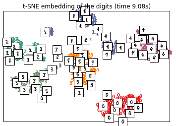
从上面的输出结果看 t-SNE 确实具有极强的流形分析能力，能够把 mnist 手写数据集这个比较复杂模式区分开来，所以这个非线性的流形学习方法能够有助于我们发现数据集内部的模式，下面使用 t-SNE 方法分析老师所给数据集是否存在某种特定的模式